Compression coefficients plot and export

Tabular Compression template provides a Plot compression coefficients feature.

Plot compression coefficients allows visualization of dependencies between compression coefficients.

This feature is available in Training section for Training Data and in Metrics section for any dataset.

The dependencies can be viewed by pairs of coefficients in 2D plots or by triples of coefficients in 3D plots. Note on special cases: naturally, when the data are compressed to a single coefficient, this feature does not exist; when the data are compressed to two coefficients, only 2D plots are available.

In Metrics section:

• Go to the Plot compression coefficients tab.

• Choose a dataset to plot among the evaluation files. Note: multiple datasets can be plotted on the same graph: right-click on the dataset that you want to add and choose “set color to coefficients plotter”

• Choose viewing parameters in Plot compression coefficients window: the dimension of the plot (2D or 3D) and the compression coefficients that you want to study among all calculated.

• You can choose to highlight and export the datapoints from the plot:

  • Put the cursor on the plot, right click and drag to plot the closed shape around points that interest you. The points inside the closed shape will become red.

  • To add more points: hold shift, right click and drag to plot a new closed shape, the points inside will be added to your selection

  • To clear selection: click Clear or right click

  • To export the datapoints selection: choose either to export only the selection markers or the selection markers with the data (the whole input or the compressed coefficients). The selection markers are described by 0/1 encoding: each datapoint in the plotted dataset is marked as 1 if the datapoint is in highlighted selection or as 0 otherwise.

This feature allows to hunt down the hidden classes of behavior in the provided data, when they exist. A toy example of such a utilization: Heaviside test case.

• The NeurEco compresses the training data from 20 inputs to two compression coefficients

• Observing the Plot compression coefficients, one can notice that the datapoints are grouped in visually distinct groups

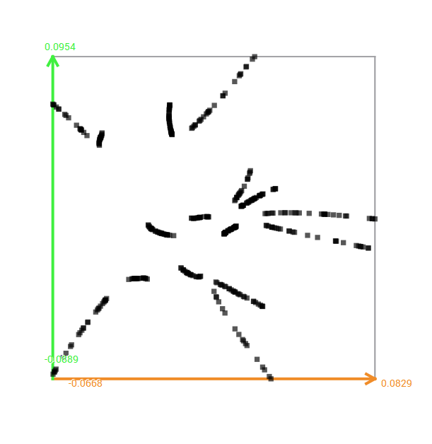
Compression coefficients of Heaviside test case

• Select and export every group, they are 16

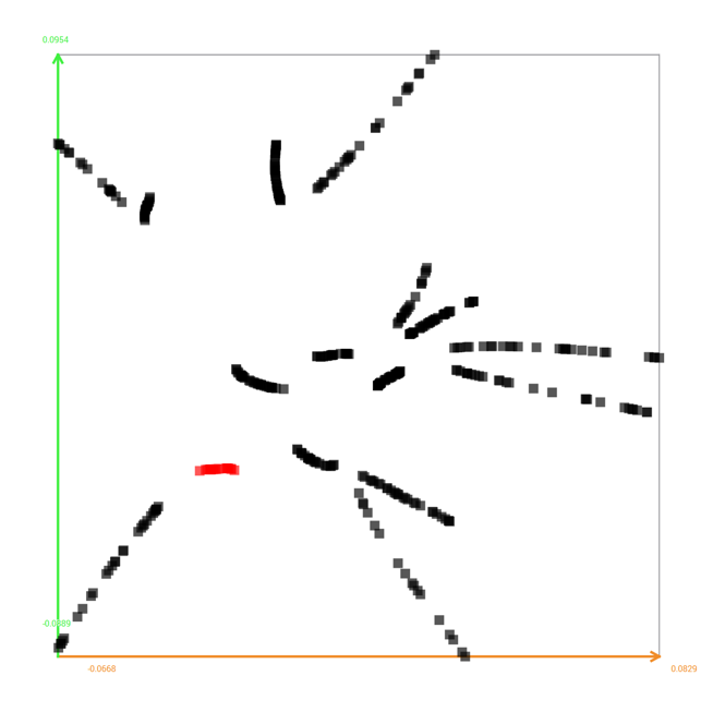
Select one group of datapoints to export

• Observing the input data corresponding to each exported group, one can quickly notice that the datapoints in the same group has the same coordinate of the jump in the Heaviside function.

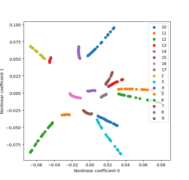
Compression coefficients for Heaviside test case. The numbers in the legend correspond to the coordinate of the jump.

NeurEco Compression discerned the groups of behavior present in the data.